 BatteryRam
Using statistics to prove randomness of a sample.
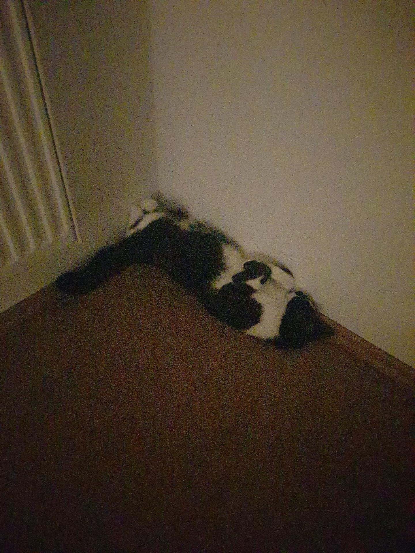
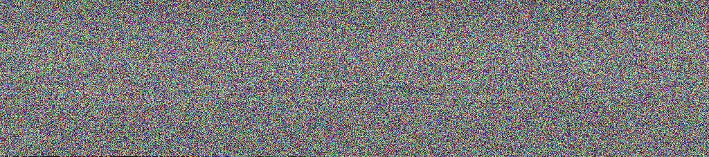
To start off the talk about randomness, let me ask you the following question: Which of the following images can be considered random?
But first, what is “randomness”? Randomness is the the inability for something to be explained by patterns or trends. Your ability to read this sentence is due to the fact that it follows the gramatical structure defined by the language. On the other hand, it is very much possible to break away from the pattern, like my inclusion of a second “the” in the second sentence of this paragraph, which, admittedly, is kinda random, is it not?
But this is not the type of randomness that I want to explore in this post. What I do want to explore is randomness of numbers. After all, the tool I wrote allows you to test whether you classify as a random number generator. If that is not what brought you to this blog post, you may view it here. I have to admit that I was never really a math nerd, but doing statistics in R during my previous semester in university was quite fun. This is what inspired me to try to learn more about this subject and ultimately, create the randomness tester. So, how does this tool actually work?
This tool uses 3 tests that we used during class to verify randomness:Wald-Wolfowitz Runs Test, Turning Point Test and Bartels’ Rank Test. All of the aforementioned tests return a statistic calculated based on the observed value from the test (the number of ranks, the number of turning points and the Von Neumann Ratio respectively), the expected mean and the expected variance (expected assuming the sample is random).
After I calculate all the statistics, I use them to calculate the p-value, which is the probability of this sample occuring naturally, assuming that the generator is indeed random. All the tests I used inside this tool follow the Normal Distribution, a.k.a the Bell Curve, which made my job significantly easier, since I could use the same function to calculate the p-value for all the tests.
Now, if you, reader, thought to yourself: “I want to verify whether this guy’s project is legit” and used an actual statistics program or the implementations of those functions in the R programming language, you would find that the p-values differ slightly. The reason for that is I use perhaps the easiest method to calculate the p-value and that is to look it up in a Z-table. From what I read, R calculates the p-value directly using the Cumulative Distribution Function, which uses the exact values of the statistic and not rounded to 2 decimal places, like I have to do in order to look it up in the table. Hence the discrepancy. Perhaps one day I will improve upon the test, but for now, the table stays.
Returning to the explanation. After I calculate the p-values for all the tests, I use a simple score system tO determine the final verdict. The scores are given as follows:
- If the p-value of the test is less than 0.05, the score is -1 (the test is considered not passing)
- If the p-value of the test is between 0.05 and 0.1, the score is 0 (the test is considered barely passing)
- If the p-value of the test is higher than 0.1, the score is 1 (the test is considered passing)
Now, why did I chose those bounds. As some people familiar with statistics may recognize, 0.05 is a very common threshold of significance of the primary hypothesis (or null hypothesis as many call it). Basically, statisticians generally agree that if the p-value is greater than 0.05, then the test is considered passing. Otherwise, the test fails. If you want to read a bit more, check out this article. I think it explains it pretty well. On the other hand, we have 0.1, which I use for the “upper bound”, so to speak. This is based on my own experience with statistical tests that I had during my class in university. In some rare cases we would have a dataset that did just barely pass the tests, but once you looked at the graphical representation, you could see that there is in fact a bit of a trend. Which is why instead of the usual “fail/pass” approach, I decided to also add “barely passing”, to make the results of the test a bit more verbose.
After scoring individual tests, I tally up all the scores and grade the overall result:
- 3 = unanimously random
- 2 = very much random
- 1 = quite random
- 0 = acceptably random
- -1 = just barely random
- -2 = not random
- -3 = unanimously not random
I think this approach will allow more people without a mathematical background to check out the test and be able to interpret the results or even give an opportunity to experiment with different samples to see how far they can push this tool.
Now, onto the question I posed at the very beginning of this post. If you look at the first image, you may recognise a picture of a cat. My cat to be more precise. I thought she looked really cute when she was lying in the corner of my room one evening so I took a picture. Considering it is possible to recognise a cat in the picture this means that this picture is not random. What about the second? “He probably used some random number generator to generate a long sequence of numbers and turned it into an image.” is what you might have thought as you proclaimed that this is a random image. Surprisingly, neither of those images are random. If you have figured it out and found out why before reading this, congratulations. If you have not, then here is solution. The second image is actually the first image…. turned into an image. Or more precisely, a compressed image treated like an uncompressed image. Basically, I took the entire file with the first image (including the part that tells the computer to treat this file like a JPG, called a JPG header) and copied it into a file with a BMP header (that tells the computer to treat this like a BitMap, which is one of the simplest image formats to process). If you remove the first 58 bytes of the second file and save the rest as an image, you will find a copy of the first image. So as you can see, seemingly random things might just not be as random as you think.
edit 17.08.26
Apparently, Neocities does not allow BMPs on the free version. So this funky little trick I mentioned will not work with the image you get on the site. Bummer. I will provide the original BMP in a github repository with the project files.
So, summing this whole thing up, I can say I had fun working on this. I was surprised to see how simple those tests ended up being. When I initially encountered them, I though to myself that those are probably some ultra-convoluted black boxes that only some great minds like Euler or Ramanujan could understand. But even I, with my relatively average knowledge of mathematics (at least for a CS student), was capable of understanding this and it brings me a dose of satisfaction. One thing that does bug me about all this is how I calculate p-values. Perhaps one day I might dig into how actual statistics programs do it and include it inside this tool, but that is a problem for another day.